Chapter 41 — The Circular Flow of Income
Cambridge International AS & A Level Economics (9708) · Unit 9.1 · 4th edition coursebook
Learning objectives
- explain the meaning of the multiplier
- calculate the multiplier using formulae in a closed economy without a government sector, a closed economy with a government sector and an open economy with a government sector
- calculate the average and marginal propensities to save, consume and import
- calculate the average and marginal rates of tax
- analyse how national income is determined, using aggregate demand and income approach
- calculate the effect of changing aggregate demand on national income using the multiplier
- describe the determinants of aggregate demand
- explain the consumption function: autonomous and induced consumer expenditure
- explain the savings function: autonomous and induced savings
- explain the determinants of investment
- explain the difference between autonomous and induced investment
- explain the meaning of the accelerator
- analyse the determinants of government spending
- describe the determinants of net exports
- explain the relationship between the full employment level of national income and the equilibrium level of national income
- analyse inflationary and deflationary gaps.
Key terms
- multiplier
- a numerical estimate of a change in spending in relation to the final change in spending.
- marginal propensity to save (mps)
- the proportion of extra income which is saved.
- marginal propensity to consume (mpc)
- the proportion of extra income that is spent.
- aggregate expenditure
- the total amount spent in the economy at different levels of income.
- marginal propensity to import (mpm)
- the proportion of extra income spent on imports.
- consumption
- spending by households on goods and services.
- average propensity to consume (apc)
- the proportion of income that is consumed.
- average propensity to import (apm)
- the proportion of income that is spent on imports.
- consumption function
- the relationship between income and consumption.
- savings function
- the relationship between income and saving.
- autonomous investment
- investment that is made independent of income.
- induced investment
- investment that is made in response to changes in income.
- accelerator theory
- a model that suggests investment depends on the rate of change in income.
- capital-output ratio
- a measure of the amount of capital used to produce a given amount, or value, of output.
- inflationary gap
- the excess of aggregate expenditure over potential output (equivalent to a positive output gap).
- deflationary gap
- a shortage of aggregate expenditure so that potential output is not reached (equivalent to a negative output gap).
41.1The multiplier
The multiplier describes the relationship between an initial change in spending and the larger final change in GDP that follows. It is sometimes called the national income multiplier. The mechanism is straightforward: an injection of spending creates income for those receiving it, and part of that income is spent again, generating yet more income for somebody else. The process continues — each round smaller than the last — until the total increase in withdrawals matches the original injection. The multiplier can be measured after the event as the ratio of the change in income to the change in injection, or estimated in advance using the formula 1 / marginal propensity to withdraw (see Figure 41.5).
Key concept link — Equilibrium and disequilibrium
The greater the size of the multiplier, the greater the change in national income as a result of an injection.
The multiplier and equilibrium national income in a closed economy, a closed economy with a government sector and an open economy with a government sector
Economists build the multiplier model in stages, starting with the simplest economy and adding sectors one at a time.
Closed economy
A closed economy contains only households and firms. There is one withdrawal — saving (S) — and one injection — investment (I). The multiplier can be written as 1 / mps, where mps is the marginal propensity to save. Because in this model income is either spent or saved, the multiplier can equivalently be written as 1 / (1 − mpc), where mpc is the marginal propensity to consume. The mpc is the change in consumption divided by the change in income, and the relationship 1 − mps = mpc holds throughout. Equilibrium income occurs where aggregate expenditure equals output (C + I = Y) and injections equal withdrawals (I = S).
Closed economy with a government sector
Adding a government adds one new injection — government spending (G) — and one new withdrawal — taxation (T). The multiplier becomes 1 / (mps + mrt), where mrt is the marginal rate of tax (the proportion of extra income taken in tax; sometimes called the marginal propensity to tax). Equilibrium is where C + I + G = Y and I + G = S + T.
Open economy with a government sector
The fullest model adds the foreign sector, giving four sectors in total: households, firms, the government and overseas. Equilibrium income occurs where C + I + G + (X − M) = Y and I + G + X = S + T + M. The full multiplier is 1 / (mps + mrt + mpm), where mpm is the marginal propensity to import. Because there are three withdrawals rather than one, the denominator is larger and the multiplier is smaller than in the simpler models. On the other hand there are now three injections, so there are more channels through which GDP can change.
Key concept link — The margin and decision making
The multiplier is calculated using marginal concepts which can change over time. For example, if the government raises the marginal rate of tax, the size of the multiplier will fall.
The average and marginal propensities to save
When income is very low, almost all of it has to be spent to meet current needs. Spending may even exceed income, with households drawing on past savings or borrowing — a situation known as dissaving. As income rises, some can be set aside. Saving is consumption subtracted from disposable income. The average propensity to save (aps) is the proportion of disposable income that is saved (S/Y) and equals 1 − apc. The marginal propensity to save (mps) is the proportion of any extra income saved (ΔS/ΔY). Both aps and mps tend to rise as income rises, so richer households typically have a higher mps than poorer households.
The average and marginal propensities to consume
Consumption is mainly determined by disposable income. As income rises, total spending rises too, but the proportion of income spent tends to fall. The average propensity to consume (apc) is C/Y and equals 1 − aps. Richer households therefore have a lower apc and mpc, and a higher aps and mps, than poorer households.
The average and marginal rates of tax
The average rate of tax (art) is the proportion of income taken in tax: art = T/Y. The marginal rate of tax (mrt) is the proportion of extra income paid in tax: mrt = ΔT/ΔY. The marginal rate is what matters when calculating the multiplier.
The average and marginal propensities to import
The average propensity to import (apm) is the share of income spent on imports (M/Y). It varies significantly between countries depending on the size of the economy, its industrial structure and its openness to trade. The marginal propensity to import (mpm) is ΔM/ΔY and also varies between countries and over time. As with saving and tax, it is the marginal — not the average — propensity that enters the multiplier formula.
National income determination
The level of national income is determined where aggregate demand equals aggregate supply, which is also where aggregate expenditure equals output. Aggregate expenditure is the total that will be spent at different levels of GDP and is made up of consumption (C), investment (I), government spending (G) and net exports (X − M). If aggregate expenditure exceeds current output, firms expand production, hire more factors and GDP rises. If it falls short, firms cut production and GDP falls. Output adjusts until it matches expenditure.
The relationship is often illustrated on the Keynesian 45° diagram. Money GDP is shown on the horizontal axis and aggregate expenditure on the vertical axis. A 45° line from the origin shows all points at which expenditure equals income. Equilibrium GDP is where the aggregate expenditure curve crosses the 45° line. An aggregate expenditure curve is not the same as an aggregate demand curve: AD plots total spending against the price level, whereas the aggregate expenditure curve plots total spending against the income level.
The effect of changing aggregate demand on national income
A change in total spending on a country's goods and services changes national income by the size of the injection multiplied by the multiplier. The rise occurs in stages — initial spenders earn income, spend part of it, the next recipients spend part of that, and so on — until leakages from the circular flow once again equal the size of the initial injection. A rise in saving has the opposite effect: it cuts spending, lowers GDP and can paradoxically lead to households actually saving less, because lower income reduces their ability to save.

Opening up to international trade adds imports as a new leakage from the circular flow, raising the marginal propensity to leak. Since the multiplier is 1 / (sum of leakages), a larger leakage means a smaller multiplier. The value of the economy's multiplier therefore falls — option D.
41.2Components of aggregate demand and their determinants
Households' spending depends on a range of influences. The main one is income, but the rate of interest, expectations, wealth, the availability of bank lending and the distribution of income all matter too. A higher rate of interest raises the opportunity cost of spending — saving becomes more attractive and borrowing becomes more expensive — so demand for expensive goods such as cars and foreign holidays falls. If commercial banks restrict lending, households may not be able to borrow as much as they would like even at a given interest rate. Expectations of future income matter almost as much as current income: households who expect to be better off in the future may adjust their spending now. Wealthier households can liquidate assets to fund purchases or use their wealth as collateral for borrowing. If income becomes more unevenly distributed, total consumption may fall because the rich spend a smaller proportion of their income than the poor do (see Figure 41.7).
The consumption function: autonomous and induced consumer expenditure
The consumption function shows how much will be spent at different levels of income. It takes the form C = a + bY, where C is consumption, a is autonomous consumption (the amount spent even when income is zero, which does not vary with income), b is the marginal propensity to consume, and Y is disposable income. The term bY is induced consumption — spending that depends on income. For example, if C = $100 + 0.8Y and income is $1000, then consumption is $100 + 0.8 × $1000 = $900.
The savings function: autonomous and induced saving
The savings function is the mirror image of the consumption function. It takes the form S = −a + sY, where S is saving, s is the marginal propensity to save, Y is income and −a is autonomous dissaving — the amount of savings households draw on when their income is zero (this amount does not change as income changes). The term sY is induced saving, the part of saving determined by the level of income. The function can be used to read off how much, and what proportion, households save at any income level.
Investment, autonomous and induced investment
Investment depends on changes in income (and so on consumer demand), the rate of interest, technology, the cost of capital goods, expectations and government policy. Investment can change quickly and by large amounts. A change in consumer demand has a powerful effect because firms buy capital goods in order to produce consumer goods: rising demand for output induces firms to expand capacity. The rate of interest influences investment in several ways — it changes the cost of borrowing, alters the return from holding funds in alternative uses, and affects consumer expenditure and hence the profits firms expect. Advances in technology bring new and more productive capital goods, encouraging firms to upgrade; a rise in the price of capital goods has the opposite effect. Expectations are a major reason investment is so unstable: a pessimistic forecast from a credible source can cause firms to delay capital spending sharply. Government policy influences investment through corporate tax rates, subsidies and income tax changes that alter consumer spending power.
Autonomous investment is undertaken independently of income — perhaps because a firm has become more optimistic, or because interest rates have fallen. An increase in autonomous investment shifts the aggregate expenditure line upward and raises GDP by a multiple amount through the multiplier. Induced investment, by contrast, depends on changes in income and shows up as a movement along the expenditure line: as income rises, firms add to their capital stock to meet the higher demand, but only continue to do so if GDP keeps rising.
The accelerator
The accelerator theory focuses on induced investment and emphasises the volatility of investment. It states that investment depends on the rate of change in income (and therefore consumer demand), and that a change in GDP causes a more than proportionate change in investment. If a rise in GDP causes induced investment to rise by a larger amount, the accelerator coefficient is 3.
If GDP grows at a constant rate, induced investment does not change — firms simply buy the same number of machines each year to expand capacity. But if the rate of growth itself changes, investment can swing sharply. A rise in the growth rate of consumer demand can produce a much larger percentage rise in demand for capital goods; a slowdown in the growth rate can cause investment to fall even when consumer demand is still rising; and a fall in consumer demand can make investment fall to zero, with worn-out machines simply not being replaced, so that productive capacity is reduced. The accelerator does not always work cleanly, however. Firms with spare capacity will not invest in response to higher demand; firms that doubt the rise will last will hold back; capital goods industries themselves may already be running at capacity; and advances in technology can change the capital-output ratio, so that fewer machines are needed for a given output.
Government spending
Government spending may rise during an economic downturn in an attempt to prevent a recession — extra spending is injected into the circular flow to support aggregate demand, maintain employment and lift output. Government spending as a share of GDP tends to be higher where the government believes there is significant risk of market failure: such governments are more likely to provide state-financed education and healthcare. Within these areas, advances in technology can push spending up — schools want to update IT facilities, hospitals want to buy equipment for more complex procedures, and that equipment usually requires more expensive aftercare. Changes in population also matter. A fall in the death rate raises demand for medical care for the elderly; net immigration may raise demand for state-financed housing while also providing extra tax revenue if the immigrants find work. Natural disasters and military conflicts both push government spending sharply higher.
Net exports
Net exports are driven by the relative price and quality competitiveness of the country's products and by incomes at home and abroad. Price competitiveness is in turn influenced by relative productivity, the relative inflation rate and the exchange rate. A country whose productivity is growing faster than its competitors', whose inflation rate is lower, and whose exchange rate is falling is likely to become more price-competitive and so see net exports rise. Quality competitiveness usually improves with higher net investment and better educational standards. When other countries' GDP rises, a country's purchasing power abroad rises with it, so exports tend to rise — especially if the country produces goods with a high income elasticity of demand. As a country's own income rises, however, its imports rise too, so the effect on net exports depends on the balance of these forces.
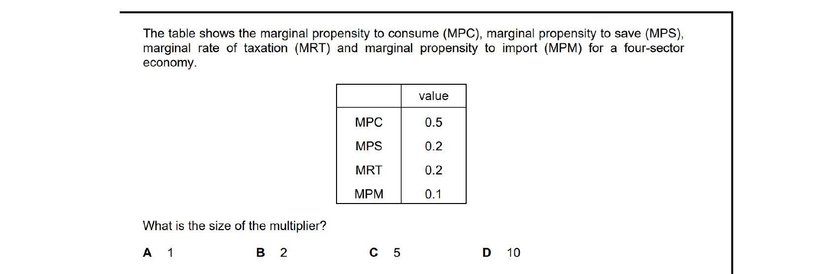
In a four-sector economy the multiplier is k = 1 / (mps + mrt + mpm). Substituting the table values: 1 / (0.2 + 0.2 + 0.1) = 1 / 0.5 = 2 — option B. (Note that MPC of 0.5 is consistent: 1 − 0.5 = mps + mrt + mpm.)
41.3Full employment level of national income and equilibrium level of national income
Economies do not often operate at the full employment level of national income. At any particular time, they may be producing where total spending is above or below the level needed for national income to equal potential output. The equilibrium level of national income — the point where aggregate expenditure equals output, shown on the Keynesian 45° diagram as the intersection of the aggregate expenditure schedule (C + I + G + (X − M)) with the 45° line — can lie either above or below the full employment level of national income (see Figures 41.3, 41.4, 41.9 and 41.10).
Inflationary and deflationary gaps
In the short run, and according to Keynesians possibly also in the long run, an economy may fail to achieve full employment. An inflationary gap occurs if aggregate expenditure exceeds the potential output of the economy. In such a situation not all demand can be met because there are not enough resources to do so. The excess demand drives up the price level. On the Keynesian 45° diagram, the economy is in equilibrium at a level of money GDP that lies to the right of the full employment level of output. The inflationary gap is the vertical distance between the aggregate expenditure line and the 45° line measured at the full employment level of output — it shows by how much aggregate expenditure would have to fall for total spending to equal full employment output.
Closing an inflationary gap
A government may seek to reduce an inflationary gap by cutting its own spending and/or raising taxation in order to reduce aggregate expenditure. The aggregate expenditure schedule shifts down, and equilibrium money GDP falls back towards the full employment level. The size of the cut in government spending required to close the gap depends on the value of the multiplier — a small change in spending will produce a larger change in equilibrium GDP, so the necessary policy change is the size of the inflationary gap divided by the multiplier.
Deflationary gaps
The equilibrium level of GDP may instead be below the full employment level. In this case there is said to be a deflationary gap. A lack of aggregate expenditure results in an equilibrium level of GDP below the full employment level. The deflationary gap is the vertical distance by which aggregate expenditure falls short of the 45° line at the full employment level of output — it measures the rise in aggregate expenditure needed to reach full employment.
The Keynesian solution to a deflationary gap
The Keynesian solution to a deflationary gap is increased government spending, typically financed by borrowing. The aggregate expenditure schedule shifts upward, raising equilibrium money GDP. The required injection is, again, the size of the gap divided by the value of the multiplier. Because the multiplier process amplifies an initial change in spending, even a modest increase in government expenditure can in principle eliminate a deflationary gap, provided households and firms respond as the model predicts.
The analysis assumes that the price level is fixed up to full employment, which is the central Keynesian assumption underpinning the 45° diagram. Once the economy reaches full employment, any further increase in aggregate expenditure spills entirely into higher prices rather than higher real output. Inflationary and deflationary gaps are therefore the Keynesian equivalent of positive and negative output gaps in AD/AS analysis, and they form the basis for demand-management policy in this framework.
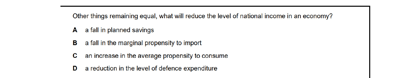
Government spending is an injection into the circular flow, so a reduction in defence expenditure (option D) directly cuts an injection and lowers national income via the reverse multiplier. The other options either raise an injection, reduce a leakage, or increase the multiplier — all of which would raise, not reduce, national income.
End-of-chapter practice
Past-paper questions from CIE 9708. Pick A, B, C or D. Answers are saved on this device — press Download report (PDF) at the top to save them.
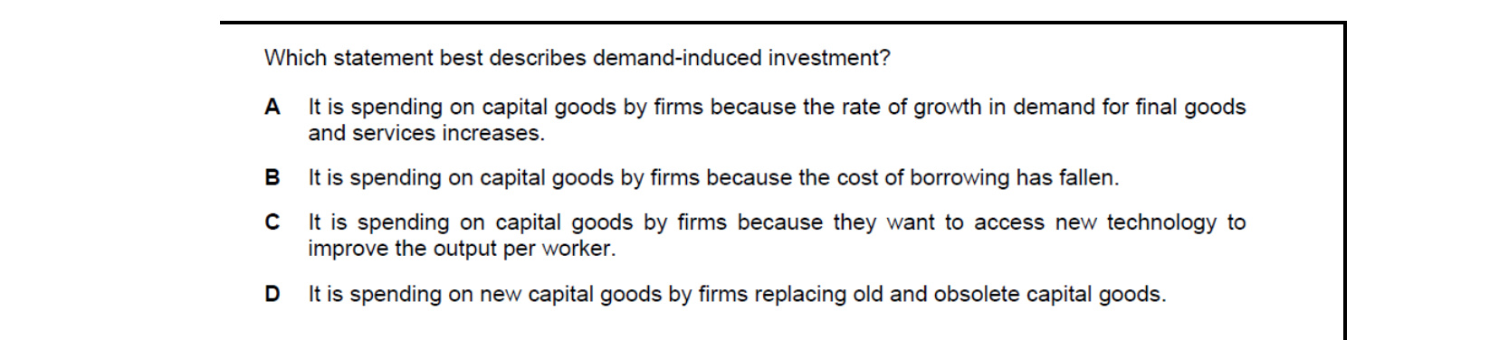
Demand-induced (induced) investment is investment caused by changes in the demand for final goods, in line with the accelerator principle. Spending on capital goods because the rate of growth of demand for final goods is increasing (option A) is the textbook example; the other options describe autonomous, technology-driven or replacement investment.

The multiplier in an open economy with a government sector is 1 / (mps + mrt + mpm). Inserting the figures: 1 / (0.2 + 0.3 + 0.3) = 1 / 0.8 = 1.25 — option A. The three marginal leakages sum to 0.8, so each extra dollar of injection raises Y by $1.25.
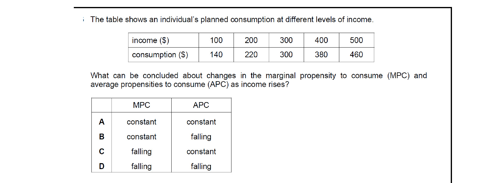
With a linear consumption function C = a + bY (a > 0), the marginal propensity to consume b is constant — extra units of income always change consumption by the same fraction. But the average propensity to consume C/Y falls as Y rises because the fixed autonomous component a is spread over a larger income. The combination is MPC constant, APC falling — option B.
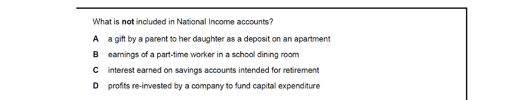
National income measures payments for productive activity. A gift from one person to another (option A) is a transfer payment — no new good or service is produced — so it is excluded. Earnings, savings interest and reinvested profits all represent income from current production and are included.
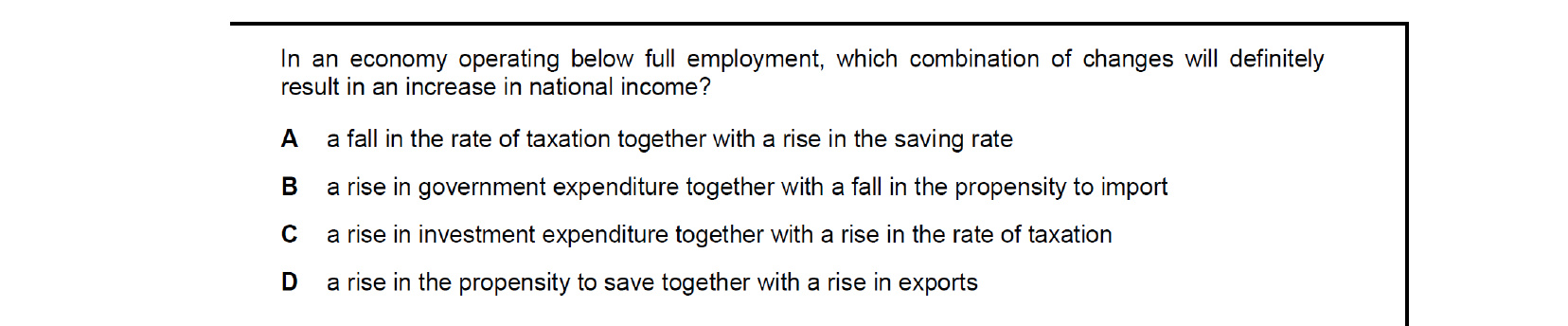
Below full employment, output rises when injections rise or leakages fall. A rise in government expenditure (an injection) and a fall in the marginal propensity to import (a smaller leakage, so a larger multiplier) (option B) unambiguously increase national income. The other options combine offsetting changes whose net effect on Y is uncertain.

With households spending 80% of income, mpc = 0.8 and mps = 0.2, so the multiplier is 1 / 0.2 = 5. To close the deflationary gap, GDP must rise by $1200bn − $1000bn = $200bn. The initial change in aggregate demand needed is $200bn / 5 = +$40bn — option C.
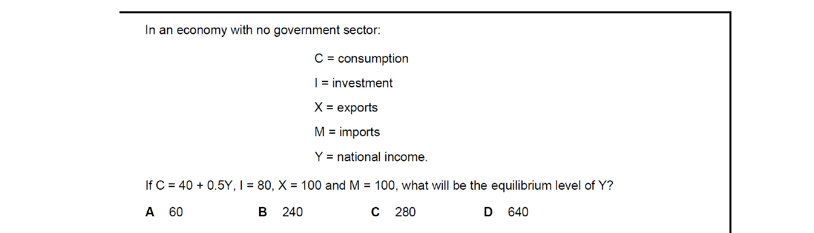
In equilibrium Y = C + I + (X − M) = 40 + 0.5Y + 80 + 100 − 100 = 120 + 0.5Y. Solving 0.5Y = 120 gives Y = 240 — option B. (Equivalently, autonomous spending of 120 multiplied by k = 1 / 0.5 = 2 gives the same answer.)
Attempt the practice questions above to build your score.
Self-evaluation checklist
After studying this chapter, you should be able to:
- Understand that the multiplier shows the relationship between an initial change in spending and the final rise in GDP
- Calculate the multiplier in a closed economy without and with a government sector and an open economy with a government sector
- Calculate the average and marginal propensities to save (aps/mps), consume (apc/mpc), import (apm/mpm)
- Calculate the average and marginal rates of tax (art/mrt)
- Understand that national income in an economy is determined where AD = AS and aggregate expenditure equals output
- Calculate the effect of changing aggregate demand (AD) on national income using the multiplier
- Describe the determinants of aggregate demand: disposable income, wealth, the rate of interest, expectations, availability of bank loans, the distribution of income
- Explain the consumption function: autonomous and induced consumer expenditure
- Explain the savings function: autonomous and induced investment
- Explain that the accelerator theory states that the level of investment depends on the rate of change in GDP
- Analyse the determinants of government spending: the level of economic activity, the extent of market failure, changes in population, natural disasters and military conflicts
- Describe influences on net exports: changes in relative productivity, inflation rate, exchange rate, incomes at home and abroad
- Explain the relationship between the full employment level of national income and the equilibrium level of national income
- Explain that an inflationary gap will occur if aggregate expenditure exceeds the full employment level of national income, while a deflationary gap occurs when aggregate expenditure is too low to achieve full employment
Want more practice? Drill this chapter's past-paper MCQs (122 questions) →